StrataBugs 3.0 pre-release available
We have made available a pre-release version of StrataBugs 3.0 to allow interested users to help us test the system ready for release. Many of you have have previously expressed an interest in testing the new features, but we also need to make sure the existing functionality is unaffected with all the changes we have made.
If you are a StrataBugs user and entitled to a v3.0 licence, you can download the test release. Some of you will already have a v3.0 licence, others might need to contact us to get an updated licence file.
In this phase, we want to ensure that the changes to the database (the data model) do not require further changes before the full release, so we cannot guarantee that the database structure will stay the same as the final release. We therefore ask that any data you wish to work on are copied out of, or back into your existing 2.1.1 database, so that your database can be converted again when we provide the full production release.
To get started with v3.0 go to the download page and follow the instructions. Open the Help, and the learning trail for v3.0 to see a brief description of the new features. Currently we do not have a download bundle for Mac users, this will be available shortly.
The learning trail and the rest of the documentation still require further work, most of the help still relates to v2.1.1.
During the pre-release phase we will be making incremental update releases on a regular basis. Once we have reached the point of a production release, we will fix the data model for v3.0 but the applications will continue to be updated as part of our continuous product development. This means that once released, you will be able to convert your database to v3.0 and it will not need further conversion until we release v3.1.
Thank you for your patience.
Should groups contain only unique taxa?
Taxon groups in StrataBugs can contain any number of species (or genera, since v2.1). Groups can be added to a Group Set, which allows the relative proportion of the taxa in each group to be plotted, often in the form of compact “closure” diagrams that show stratigraphic or environmental trends. So far so good. We’ve pretty much assumed that, up until now, a Group Set will contain an exclusive set of taxa; i.e. each taxon will only occur in one group, when that group belongs to a Set. Indeed, when you create or edit a Set in the Taxonomic Database module, it warns you if there is any duplication between the groups, and allows you to see the duplicates:
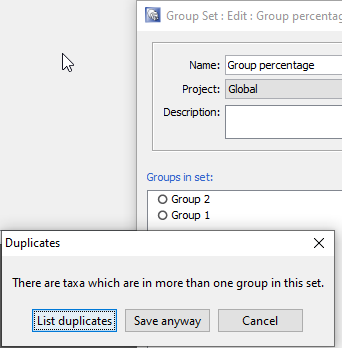
But what happens when a taxon belongs to more than one group in the Set? What if you have groups that reflect broad environmental conditions, and some taxa are present in a range of environments which spread across more than one group? To display these groups as a relative abundance curve would be to double count the abundance of taxa in each group. But to include them in some groups and exclude them from others seems arbitrary. Up until now, the latter is what has happened in the v2.1 charts, and this has been inconsistent with the previous behaviour in the “legacy” charts. In the “legacy” charts, each taxon was added to the total for each group, so if a Group Set was plotted with relative group abundance, those groups with duplicate taxa would be more heavily weighted compared to the other groups. In the v2.1 charts, the taxon is only counted once – but this has the distorting effect of ignoring the influence of the taxon in any subsequent group it might appear in.
I think a better solution exists than either of these scenarios. If a taxon exists in more than one group, then perhaps the weighting of that taxon’s abundance should reflect the number of groups that it is spread between. So if it occurs in two groups, then 50% of the count gets allocated to each group. We have just updated the v2.1.1 (and v2.1.1-14) release to reflect this new thinking.
Let’s look at a simple example to illustrate the change. Suppose we have two groups; Group 1 and Group 2. Group 1 contains one taxon (Ammonia spp.); Group 2 contains 2 taxa, Ammonia spp. again, and Elphidium spp. Both taxa are recorded in an analysis, each with a count of 10 specimens. The total count is 20 specimens. Let’s start by plotting this in the legacy chart application:
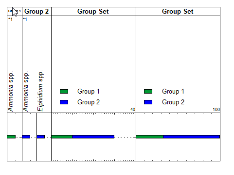
The first panels, Group 1 and Group 2 plot as expected: an abundance of 10 for each specimen. No problem there. In the third panel, showing the Group Set, the duplicate taxon in Group 2 is counted twice, so although the panel looks reasonable, the total count displayed here is 30 – whereas the true total count is only 20. The fourth panel, the relative abundance of the groups within the Set, also looks quite reasonable, but the proportions don’t correctly reflect the proportions of the contents of the groups.
Now we plot the same data in the unmodified v2.1 charts:
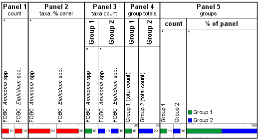
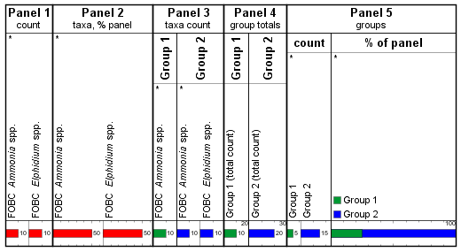
Panel 1 shows the individual taxon abundance; Panel 2 shows the abundance of each taxon as % of the total. Panels 3 and 4 have inner panels for each group, and show the count of individual taxa in the group and the group totals respectively. Ammonia spp. contributes to the count in both groups. The inner panels in Panel 5 each show the Group Set, divided by its constituent groups. Now we see an equal count (and % distribution) of Groups 1 and 2, because Ammonia has been counted in Group 1, and isn’t counted again for Group 2. This is different to the “legacy” chart above, but still does not accurately reflect the group proportions.
Worse, when we rearrange the Set’s group order, so that Group 2 is now plotted first, we see Group 1 disappearing completely in Panel 5:
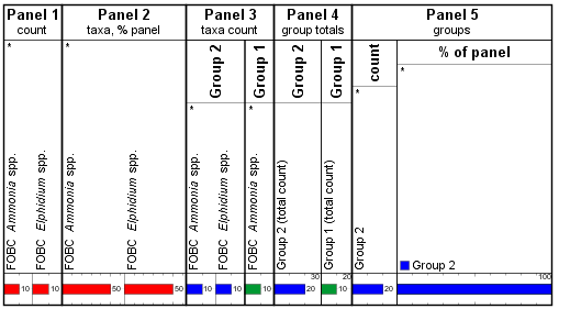
In the modified version which is now released, we divide the abundance between split groups, so we get this:
Panels 1-4 are the identical, but Panel 5, which shows the Group Set as a whole, has the 10 counts of Ammonia split between Groups 1 and 2. This means the total of the absolute abundances is (correctly) 20, and Group 1 only has 25% of the weight (as opposed to 33% in the legacy charts, and 50% – 0% in the previous version). The proportions remain the same when the groups are reordered. This also highlights the subtle but important distinction between plotting separate inner panels for each group (as in 3 and 4) compared to separate tracks for each group (as in each inner panel in Panel 5).
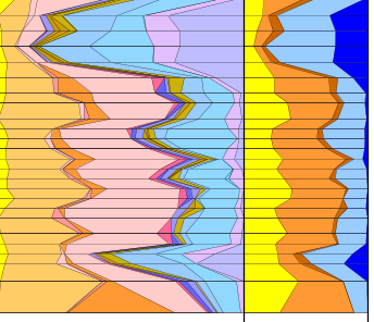
Finally, a real world example. This Group Set contains several hundred species which are ranged across different water depths. The left panel reflects unique group assignments: taxa ranging across environments are assigned to a group which exclusively contains taxa of the same range. It is difficult to get the group ordering right, with overlapping ranges, and the colour assignments can subtly affect the visual result. In the second panel, where there are fewer groups but taxa can occur in multiple groups, the deeper water depths are under represented.
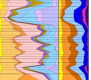
When we display the same panels with the modified version, we see a more even spread across the main groups:
This issue only affects you if you use overlapping groups, so may not be a big deal, but perhaps some explanation of what’s going on here is useful, and it can be an opportunity to more easily group taxa for displays of this kind.
Your head’s probably spinning by now and you probably wish you’d never started reading this, but if you’ve lasted out until the end, and feel the urge to comment, we’d welcome any feedback.
Saving sessions, and clicks
Those of you that typically use the “Restore Session” option when reopening the Samples & Interpretations module will have noticed that although the previous sessions wells/outcrops and tabs are restored, it didn’t reinstate the previous tab selections. This hasn’t seemed to us to be a very big deal, as we assumed that most people, most of the time, tend to work more intensively on fewer wells, so the task of clicking on a few tabs to get back to the block template you were last viewing, seems trivial.
The assumption doesn’t hold true for larger field review studies, or for shallow borehole geotechnical work which typically involves tens of boreholes (the usual scenario for BioChron). In these cases, being able to reopen your session with the same tabs open can save a lot of clicks. If this applies to you, then an update to the latest release of v2.1.1 or v2.1.1-14 is all you need to do.
If you do restore a session but get an error message pop up during the restore, then copy this to us (as always) with a simple screen shot, but don’t worry unduly because an error in this phase is unlikely to need anything other than a few extra clicks to get back to where you were.
GNATTS off to BP
Note: if you’re receiving this for the first time, you’ve just been added to our blog list. You can unsubscribe if you’d rather not receive these, but we hope you’ll find the occasional post interesting.
Waiting for a timescale is like waiting for a bus in the rain. You wait for ages, then two come along at once. We are pleased to be able to share with you a data pack of schemes based on the BP Gulf of Mexico Neogene Astronomically Tuned Time Scale (GNATTS) published in 2019. The full background and reasoning for the scale are available under open access here:
Bergen, J. A., Truax III, S., de Kaenel, E., Blair, S. A., Browning, E., Lundquist, J., Boesiger, T. M., Bolivar, M. & Clark, K. (2019). BP Gulf of Mexico Neogene Astronomically-Tuned Time Scale (BP GNATTS). GSA Bulletin, 131 (11-12): 1871-1888.
GSA Bulletin; November/December 2019; v. 131; no. 11/12; p. 1871–1888; https://doi.org/10.1130/B35062.1; 7 figures; 7 tables; Data Repository item 2018407; published online 16 April 2019.
Data are available at http:// www .geosociety .org /datarepository /2018 or by request to editing@ geosociety .org.
We have taken all the zonation schemes and events, and turned them into an updated set of biozone schemes and composite standards, which are linked to corresponding named taxa. You can download the entire set of schemes which make up this chart and import them and reconstruct this chart if you wish. Alternatively you can just import selected schemes.
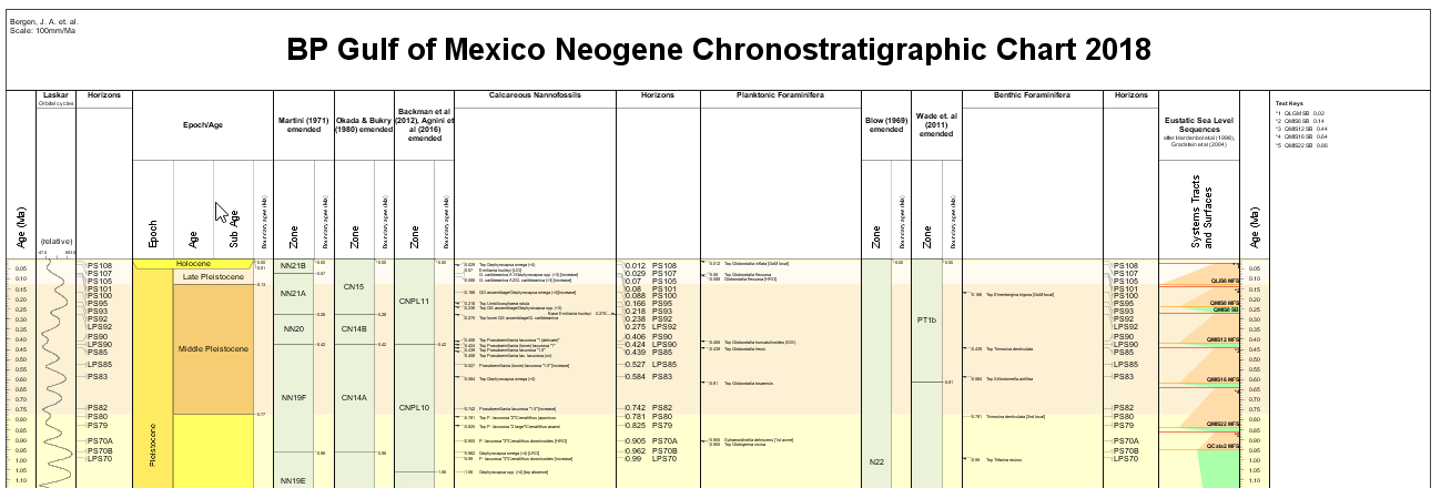
If you download the entire data pack you can import/match the linked taxa against your own data. A word of warning: the vertical scaling is based on GTS2012/2016 ages except that the Gelasian is included in Pliocene, making the Pliocene/Pleistocene boundary younger when compared to those published schemes (and indeed the standards ICS chart).
You’ll need StrataBugs 2.1 to read this file, preferably v2.1.1. use Help | About to find out which version you’re running, and contact us if you need help upgrading.
The Nannofossil events are differentiated on the basis of size, and this has been carried through to the taxonomy, to create separate species for the different size fractions. The µ symbol (for micron) is implicit in these taxon names: this is to follow the convention of the published chart, but also there is a quirk that a name search in StrataBugs will not pick up taxon names which include the µ symbol, because of the inconsistent way the uppercase character is handled in SQL.
Thanks to Todd Boesiger for supplying the initial data, and to Eric de Kaenel for all his checking and comments, much appreciated.
Time for a new timescale
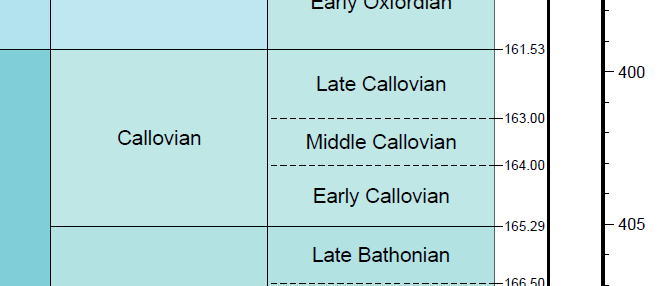
Happy new year and happy new timescale! With the publication of the new Gradstein, Ogg, Schmitz & Ogg Geologic Time Scale 2020, we have a StrataBugs friendly encoding of the new units with their updated ages and colours, which is available to download from our Schemes page. Download the .SBG file, then open Schemes & Interpretations, select Stratigraphic schemes, and press Read… to read it – then press Add Scheme to add it to your database. It will then be available for use in any charts or with well data, or just to compare against previous versions, or your favourite biozone schemes. Please let us know if you spot any errors. Note that the substages in the Cretaceous, Jurassic and Triassic are informal and illustrative. We have not recalibrated any of the “Standard” biozone schemes yet – there is a re-calibration tool in StrataBugs which allows you to do this if you wish, but this is only intended as a starting point, the final schemes should be thoroughly checked!
Note that the timescale which is available from the International Commission on Stratigraphy website, although called the 2020/v3 revision, is actually based on the previous GTS2012 timescale, so don’t get confused! We have called the previous version of this timescale “ICS” to avoid this.
GTS2016 Calibrated Transgressive/Regressive cycle sequence scheme
We’ve recently added a new calibration of the SEPM global sequence scheme for the GTS2016 time scale, featuring the terminology used in the latest version. This is available on our scheme resources page. These schemes can be simply downloaded from here and imported into your database in the Schemes and Interpretations module.
Thanks to Jake Jacovides from Millennia for preparing this version of the scheme.
If you have schemes you’d like to see, or to contribute, please get in touch, and let us know if you spot any errors.
Exporting for multivariate analysis
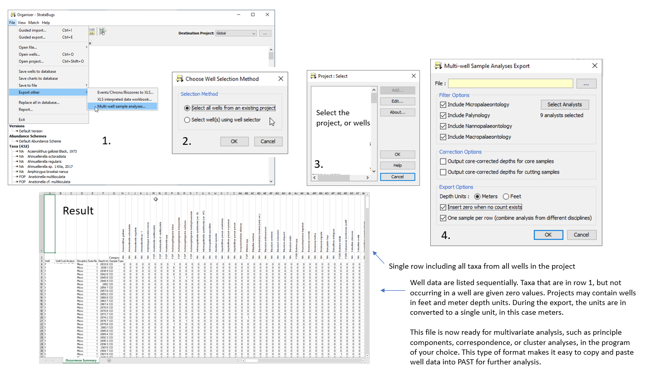
So, you have a bunch of analyses in your StrataBugs database that have, of course, been nicely QC’d and you want to do some statistical analysis. Apart from the built in clustering offered through the taxon panel, we don’t do a lot of exploratory stats like Q/R mode cluster analysis, Principal Components etc. So, you have to export the data. Up until recently, you can only export one well at a time through the “Save As” mechanism on the Analyses tab in Samples & Interpretations. This is all well and good, but what if you need to combine data from more than one well? If you export into multiple spreadsheets, then unless the fauna/flora are identical, you’re going to end up with having to manually paste in each spreadsheet carefully, so the columns all line up correctly. Major headache.
Fortunately there’s now a Multi-well sample analysis export built into Organiser, and Lawrence Febo has kindly shared this simple graphic to explain the export steps … thanks Lawrence, and enjoy …
StrataBugs and Java updates
Here at StrataData towers we’ve been working to prepare for the next major release of StrataBugs, which will likely to be called v3.0 and involve some database updates. It’s also going to be built on the latest version of Java. Things have been happening in the Java world. Many of you will have noticed that Oracle have stopped freely licencing Java except for personal use: you are now required to buy (for a nominal fee) a licence for Java itself before you can run any Java-based software. Fear not, however, as there are open source builds of Java available to download with no licensing restrictions. The current version of StrataBugs, version 2.1.1, will require version 7 or 8 of java, and there are various builds available for you to use. To simplify, we have created a downloadable bundle of StrataBugs with the Azul Zulu version of Java 8; with this you can run StrataBugs without having to “install” Java on your machine. This means that you will also not be pestered about Java updates.
We have also made available an intermediate version between v2.1.1 and v3.0, which we’re calling v2.1.1-14, which uses the latest Java 14. In this case, a tailored version of Java 14 is bundled with the download. It is fully compatible with your v2.1/v2.1.1 database, and can be used in place of your existing installation. The advantage of using Java 14 is that it responds to screen sizing better. High resolution “4k” screens are becoming more common – if you look at your Windows display properties, and it shows that your fonts etc. are displayed at 200% or 250%, then you’re likely to be running a 4k screen. In its default setting, StrataBugs will be unusable, as the contents of the windows will “outgrow” the window borders. With Java 8 there is a workaround to this: but it does look slightly pixelated. With Java 14, scaling works correctly and the windows and dialogs are sharp.
You can download this new version but you will need a licence update to run it: we are only releasing this version to current (2020) maintenance holders.
Get in touch with support@stratadata.co.uk if you want more information, or for any other StrataBugs queries.
Do your homework
These challenging times of self isolation and home working will hugely disrupt the working practices of many of you, whilst for others who already work in an office at home, your working life might remain largely unaffected by the current crisis.
For people who usually work in an office with a server based database you have a few options available to manage how you can work remotely. The strategy you choose will be based on the availability of resources and the need to integrate with others.
The basics. To run StrataBugs you will need two things: a licence and a connection to a database. There are many different configurations for both these things, and they both can either be provided centrally on a network, or to distributed stand alone machines.
The licence
We usually provide permanent licences to a server or a hardware key (dongle). In the server model, as long as you’re connected to the server and the server has a licence available, then it can be “checked out” for the duration of your session and it automoatically returns to the pool when you close. We can also extend this model to provide a licence that can be checked out from the server for a continuous period of time, up to a set limited number of days. During this period, the licence can be used independently of the network. If you look at the Control Panel Config options, and the option for “Licence check in/out from server” is not greyed out, then your licence server has this enabled. This is useful for workers due to be working off line for example at rig site where a network connection to the server is not guaranteed, but could also be used for periods of home working.
Checked out licences reduce the number of remaining licences available to others, so its use should be carefully managed to avoid people being uncessarily locked out while a licence isn’t actually required.
For individual licence holders we usually issue a dongle. This is provided with a matched licence file and has the advantage that it can be moved from machine to machine, giving the same flexibility as a server licence without the need for a network. The disadvantage is the need to have a driver installed on each machine before the dongle will be recognised.
We can also licence individual machines based on their host ID(s) which are a unique aspect of the machine’s hardware. We do not issue permanant licences for individual machines because this would remove the flexibility to transfer between multiple machines or upgrade hardware.
For these exceptional times, if you would be normally able to connect to your company licence server but are unable temporarily to do so, then we can issue a temporary licence, if you provide us with the hostid. When sending us the hostid, please copy and paste the text rather than sending a screenshot to reduce the chances of retyping it incorrectly.
The database
In StrataBugs you can set up one or more connections to databases. For most, you will only have one database that you connect to all of the time, but if that database is on a server, then when working remotely that server might be unreachable or simply too slow or intermittent to adequately work. One tip here: if you have the option, used a wired connection i.e. an ethernet cable, into your router, rather than a WiFi connection. We have found that database connections frequently get dropped when used over WiFi. Although we try to trap these instances and allow you to reconnect within StrataBugs, this isn’t always reliable.
If you find that you can’t work effectively using the remote server connection, then you can set up a connection to a local database. We use a file based database system called h2 which provides good performance for a single user. There is an h2 database called “demo” which you’ll find in the StrataBugs data folder. All the connection details for getting started with the h2 demo database are given on this page.
The demo database will obviously not contain any of the data you will have been working on in your server database. If you do need to carry on working where you left off, you have two options.
Export/Import
Firstly, before leaving the office, or if you can connect to the server remotely, you could run the Organiser module and run the guided export for all the data you’re working on. Use the default file format .sbg since this will best preserve the data for version 2.1 – older more obsolete formats like DEX have some deficiences for some data types. Save the export file to a folder location that you will be able to access offline.
When reconnected to the local database, you go through the Organiser guided import procedure, generally “adding all” as you go, and this will give you a new copy of the data into your local database that you can now work on.
Create database
There is a second option here. In the Wells and Outcrops module, there is a option for a Project (which is a list of wells and associated groups and templates) called “Create DB” which allows you to create a standalone database whch contains all of the project data. This avoids the import/merge steps of the above, but be warned, it places a heavy demand on the server and should only be run locally or over a fast enough network. It’s also sensitive to any errors in the data, so don’t be too optimistic that it will work first time! In this process, you start with an empty h2 database which just contains the table structure and some ancilliary data. See the help for a link to this database. At the end of the process you will have a file containing an h2 database which just contains your project data. One omission however is that it will not contain “Global” chart templates. See below.
Chart templates
If you use the export/import method, or you want to use global templates that the “Create database” step does not (yet) provide, you might want to also export some of your server’s global well blocks. You can do this from the “Chart/template” menu in the Charts & Templates module. If your well block uses groups and sets then these will be exported along with the panels that make up the well block. This also creates a .sbg file which you can import using the guided import of the Organiser module.
Backup
Don’t forget to backup your database file – nobody can replace this if it gets corrupted and you might lose all your data. On the connection settings there is a handy backup reminder prompt which pops up when you close the database.
Re-integration
Regardless of the method you use to get started, sooner or later you will want to get all that new or changed data back into your server database. The only option here is the reverse of the export/import method described above, except this time you’re exporting from the local database and importing back into the server database. If you have a lot of wells in your local database, remember to keep a note of which ones you’ve touched. The Oganiser guided import will allow you to see exactly what’s changed and give you the option to deal with any conflicts that arise during the merge.
As always, contact us if you need any help in managing your data.
Multi-well header loading
Many thanks to Lawrence Febo (Chevron USA) for this post…
A very useful StrataBugs feature, though perhaps overlooked, is the bulk well importer using the Organiser interface.
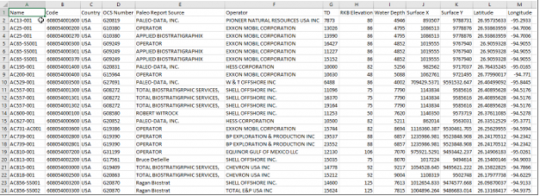
Step 1: Prepare a spreadsheet with your well header data as shown below. Four fields are required for each well (Name, Code, Location, and TD), though others can be added. In the US Gulf of Mexico, additional identifiers may be added, such as the OCS Numbers (Outer Continental Shelf).
Step 2: Choose the Organiser Module, then select File>Open file…>XLS Well headers…(Figure 2). After selecting the Excel file, you will need to select the depth units for the wells. Be sure to bulk load wells that have the same depth units. Do not import a mix of wells where some are in meters and others are in feet. If you do, then they will all go into the database in the units selected.
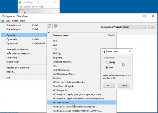
Figure 3 – View of an individual well in the list and the fields that get populated in the database.
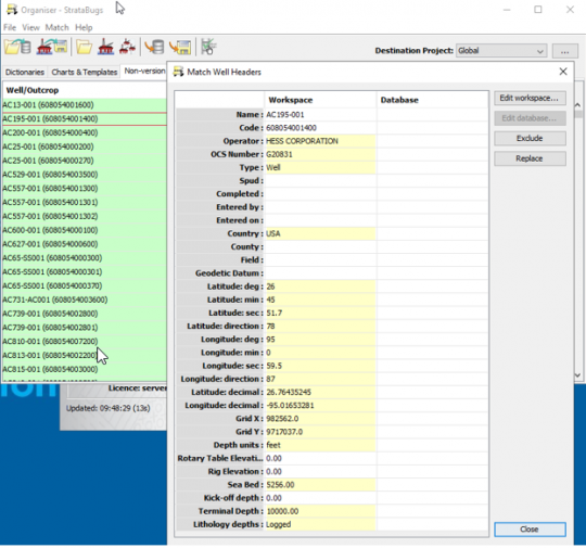
Step 3: Once the well headers are read into the workspace, the last step is to Match the wells from the workspace into the database (Figure 4). You can choose “add all” if they are all new. Figure 4 – Final steps > select “Match all” first, and then “Add all” of the unmatched wells. Any wells left unmatched will be excluded when you close the dialog.