Do your homework
These challenging times of self isolation and home working will hugely disrupt the working practices of many of you, whilst for others who already work in an office at home, your working life might remain largely unaffected by the current crisis.
For people who usually work in an office with a server based database you have a few options available to manage how you can work remotely. The strategy you choose will be based on the availability of resources and the need to integrate with others.
The basics. To run StrataBugs you will need two things: a licence and a connection to a database. There are many different configurations for both these things, and they both can either be provided centrally on a network, or to distributed stand alone machines.
The licence
We usually provide permanent licences to a server or a hardware key (dongle). In the server model, as long as you’re connected to the server and the server has a licence available, then it can be “checked out” for the duration of your session and it automoatically returns to the pool when you close. We can also extend this model to provide a licence that can be checked out from the server for a continuous period of time, up to a set limited number of days. During this period, the licence can be used independently of the network. If you look at the Control Panel Config options, and the option for “Licence check in/out from server” is not greyed out, then your licence server has this enabled. This is useful for workers due to be working off line for example at rig site where a network connection to the server is not guaranteed, but could also be used for periods of home working.
Checked out licences reduce the number of remaining licences available to others, so its use should be carefully managed to avoid people being uncessarily locked out while a licence isn’t actually required.
For individual licence holders we usually issue a dongle. This is provided with a matched licence file and has the advantage that it can be moved from machine to machine, giving the same flexibility as a server licence without the need for a network. The disadvantage is the need to have a driver installed on each machine before the dongle will be recognised.
We can also licence individual machines based on their host ID(s) which are a unique aspect of the machine’s hardware. We do not issue permanant licences for individual machines because this would remove the flexibility to transfer between multiple machines or upgrade hardware.
For these exceptional times, if you would be normally able to connect to your company licence server but are unable temporarily to do so, then we can issue a temporary licence, if you provide us with the hostid. When sending us the hostid, please copy and paste the text rather than sending a screenshot to reduce the chances of retyping it incorrectly.
The database
In StrataBugs you can set up one or more connections to databases. For most, you will only have one database that you connect to all of the time, but if that database is on a server, then when working remotely that server might be unreachable or simply too slow or intermittent to adequately work. One tip here: if you have the option, used a wired connection i.e. an ethernet cable, into your router, rather than a WiFi connection. We have found that database connections frequently get dropped when used over WiFi. Although we try to trap these instances and allow you to reconnect within StrataBugs, this isn’t always reliable.
If you find that you can’t work effectively using the remote server connection, then you can set up a connection to a local database. We use a file based database system called h2 which provides good performance for a single user. There is an h2 database called “demo” which you’ll find in the StrataBugs data folder. All the connection details for getting started with the h2 demo database are given on this page.
The demo database will obviously not contain any of the data you will have been working on in your server database. If you do need to carry on working where you left off, you have two options.
Export/Import
Firstly, before leaving the office, or if you can connect to the server remotely, you could run the Organiser module and run the guided export for all the data you’re working on. Use the default file format .sbg since this will best preserve the data for version 2.1 – older more obsolete formats like DEX have some deficiences for some data types. Save the export file to a folder location that you will be able to access offline.
When reconnected to the local database, you go through the Organiser guided import procedure, generally “adding all” as you go, and this will give you a new copy of the data into your local database that you can now work on.
Create database
There is a second option here. In the Wells and Outcrops module, there is a option for a Project (which is a list of wells and associated groups and templates) called “Create DB” which allows you to create a standalone database whch contains all of the project data. This avoids the import/merge steps of the above, but be warned, it places a heavy demand on the server and should only be run locally or over a fast enough network. It’s also sensitive to any errors in the data, so don’t be too optimistic that it will work first time! In this process, you start with an empty h2 database which just contains the table structure and some ancilliary data. See the help for a link to this database. At the end of the process you will have a file containing an h2 database which just contains your project data. One omission however is that it will not contain “Global” chart templates. See below.
Chart templates
If you use the export/import method, or you want to use global templates that the “Create database” step does not (yet) provide, you might want to also export some of your server’s global well blocks. You can do this from the “Chart/template” menu in the Charts & Templates module. If your well block uses groups and sets then these will be exported along with the panels that make up the well block. This also creates a .sbg file which you can import using the guided import of the Organiser module.
Backup
Don’t forget to backup your database file – nobody can replace this if it gets corrupted and you might lose all your data. On the connection settings there is a handy backup reminder prompt which pops up when you close the database.
Re-integration
Regardless of the method you use to get started, sooner or later you will want to get all that new or changed data back into your server database. The only option here is the reverse of the export/import method described above, except this time you’re exporting from the local database and importing back into the server database. If you have a lot of wells in your local database, remember to keep a note of which ones you’ve touched. The Oganiser guided import will allow you to see exactly what’s changed and give you the option to deal with any conflicts that arise during the merge.
As always, contact us if you need any help in managing your data.
Multi-well header loading
Many thanks to Lawrence Febo (Chevron USA) for this post…
A very useful StrataBugs feature, though perhaps overlooked, is the bulk well importer using the Organiser interface.
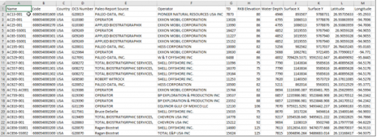
Step 1: Prepare a spreadsheet with your well header data as shown below. Four fields are required for each well (Name, Code, Location, and TD), though others can be added. In the US Gulf of Mexico, additional identifiers may be added, such as the OCS Numbers (Outer Continental Shelf).
Step 2: Choose the Organiser Module, then select File>Open file…>XLS Well headers…(Figure 2). After selecting the Excel file, you will need to select the depth units for the wells. Be sure to bulk load wells that have the same depth units. Do not import a mix of wells where some are in meters and others are in feet. If you do, then they will all go into the database in the units selected.
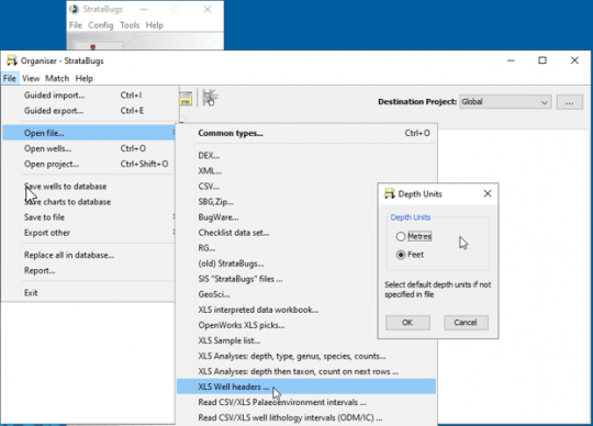
Figure 3 – View of an individual well in the list and the fields that get populated in the database.
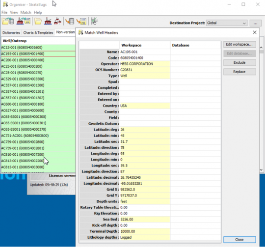
Step 3: Once the well headers are read into the workspace, the last step is to Match the wells from the workspace into the database (Figure 4). You can choose “add all” if they are all new. Figure 4 – Final steps > select “Match all” first, and then “Add all” of the unmatched wells. Any wells left unmatched will be excluded when you close the dialog.
Select this view for all open wells
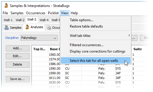
It is a common scenario to open up a project (containing many wells) in Samples & Interpretations, and want to look at the same thing in all of them. Perhaps it’s the micro analyses, the list of sequence picks in a particular version, or a particular templated chart. To save some tedious clicking we’ve added a menu option to replicate the currently selected view, as closely as possible, in all open well tabs.
Open up your project and navigate to the view you want to see in one well. Go to View > Select this tab for all open wells.
- The analysis suite filter (discipline, analyst, suite number) will be replicated for the Analyses tab.
- The version and interpreted data type tab selection will be replicated for the Interpretations tab.
- The selected chart tab will be replicated for the Charts tab, for wells which already have a tab for the same template (hint: you can use the menu option File > Open chart template tab for all wells… to initialise a chart template tab for every well in the project). The selected version is also replicated for the Charts tab.
Making taxonomy less taxing
We’ve added a new feature to StrataBugs 2.1.1 to make it easier to access some of the wonderful resources that are available on the web. The “web lookup” button has long been around on the taxon matching dialog to enable generalised Google searches on the selected taxon name, as a quick QC method before adding new species names to your dictionary.
The Nannotax/Mikrotax team have made some elements of their underlying database available via an API, which means that StrataBugs is able to query the resource directly and display results ‘in-house’, without you having to go to your browser at all. At its simplest, this gives you a way to ‘verify’ your taxonomy against external dictionaries. If you do need more information, you jump directly to the relevant page.
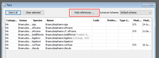
With the latest update for 2.1.1 installed, you will notice a new button on the taxa list window in the Taxonomic Database module. Take any list of taxa: this could be obtained in a number of ways, for example…
- the contents of a group – open the group, select all the taxa and drag them into the main taxon list window
- all the taxa recorded in a well or project, by using the Taxa menu search option
- using the menu item to search by date, to find all recently added taxa
Now, with the taxa list populated, you press the Web References button:
The next window will ask to confirm the data source(s) used for the lookup. Currently only Nannotax/Mikrotax is supported, but we hope that we will be able to add other APIs to the list when they become available.
Each taxon in your list will be matched to the data source. Be patient for long lists, as it is dependent on your internet connection. When the search is finished the non-matching taxa are selected (in case you want to clear them perhaps), and a new column will appear with the reference (hint: you can make this column wider by grabbing the right side of the column header and dragging to the right). In common with other StrataBugs tables, you can sort the rows by clicking on the column headers.
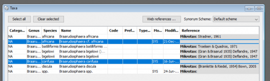
You can see that two out of my eight original species were not found in Mikrotax. If I right-click on one of the taxon entries I can select the option “Go to URL”: this opens my web browser at the relevant page for the selected taxon.
Nannotax covers most of the nannoflora, but only some of the microfossil categories are covered in Mikrotax e.g. Radiolaria. Depending on the focus of your work, this ‘reference checker’ could be a useful tool for QC’ing your database. There is potential to do more with this data – please do approach us with your ideas on what you think would be most useful. And if you are connected with other database projects that offer a web services interface (or might be interested in creating one), we can look into building similar links.
StrataBugs v2.1.1 – overriding well block templates in individual wells
Some months ago we started to work on an improvement to the new charts system to address what seemed to be a very common question: “Can I just change this panel in this one well?” The results are now available to everyone in version 2.1.1.
Recap on well block templates
A block template is an ordered list of panel templates, with captions. It is a saved design layout, usually belonging to one project, which can be used to display data from any well. It makes sense to be able create a standardised chart for each well in a project, especially where the different wells have similar data content which might be need to analysed or displayed in the same way. Because “charts” are always coupled to their templates, you can change your mind about the layout or design without having to edit a chart for every single well – just make the change to the template, and all your charts will be updated. This is far cleaner and more flexible than having separate charts for each well (as was the process in the old charts model).
So far so good, but it seems that standardisation can only go so far. Different wells have their quirks, and you need to tweak the design ever so slightly in some cases. Perhaps a different wireline log here, or a slightly different group of taxa there. In the original 2.1 charts module the only way you can do this is to duplicate the block template – probably giving it a name specific to the well for which you needed to make the tweak. Suddenly, instead of having one block template which is neatly shared around the project, you’ve got a separate “template” for each well and you’ve lost all the benefits of having templates in the first place.
New overrides feature
We wanted to allow the flexibility to tweak chart design for individual wells, whilst retaining the benefits of the template-driven model. Version 2.1.1 handles the complexities internally, giving you just a simple option to change some panel properties in individual wells, if you wish, and see those changes reflected wherever you use that template to display that well. You can still make changes to the base template and see them reflected everywhere.
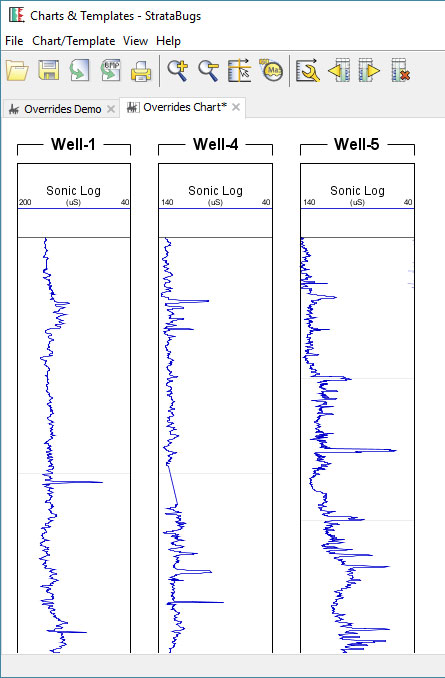
Here is a simple example. I create a well block template with one panel, showing the sonic log. I create a new chart and add some blocks for wells in my project, using my new template.
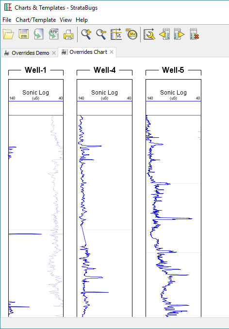
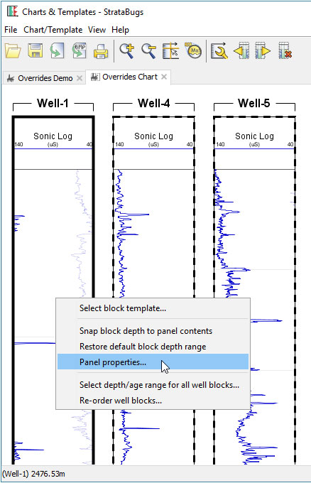
The horizontal log scale looks fine for Well-4 and Well-5, but it’s not great for Well-1. Previously I would have had to make a compromise and decided on a scale which I could use for all wells (or create a separate well block template just for Well-1). With v2.1.1 I can right-click on the panel in Well-1 and select Panel Properties:
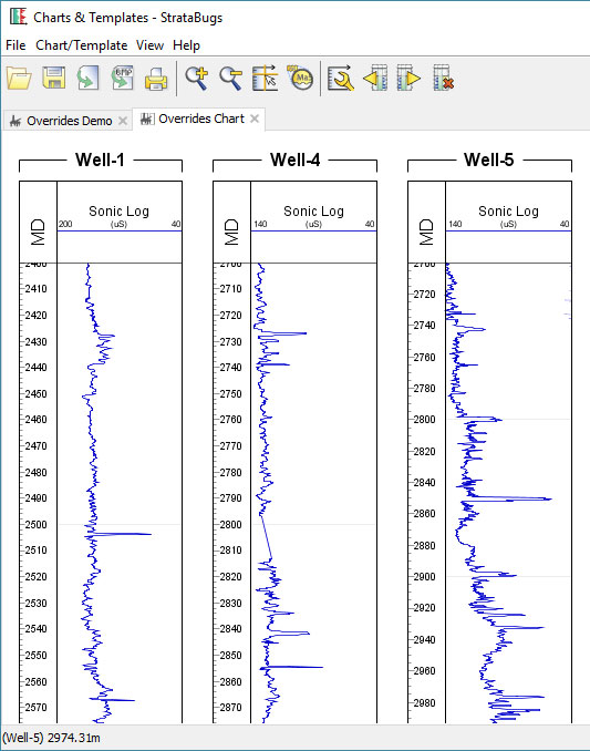
After adjusting the DT (sonic) scale, my chart is looking better.
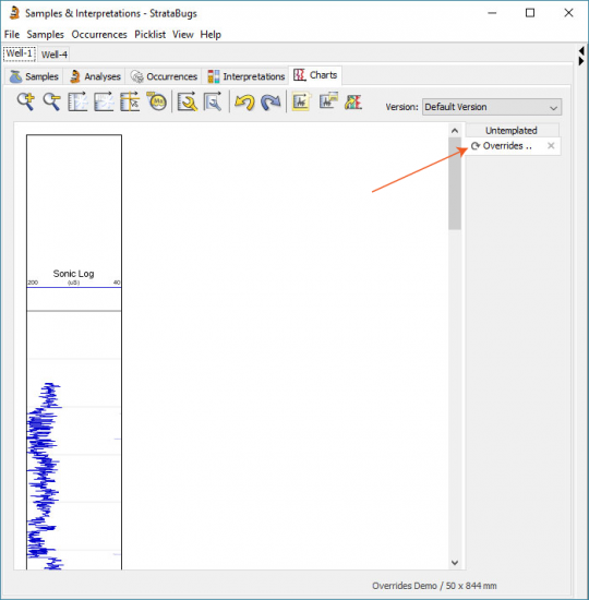
When I have saved this chart, my override for this panel for Well-1 will be saved and applied whenever else I open this template for Well-1. So if I open a tab for it in Samples & Interpretations, my new scale applies. An arrow symbol in tab indicates that this block template has panel overrides in this well.
If I make a change to the block template, e.g. I add a depth scale panel, it updates for all wells.
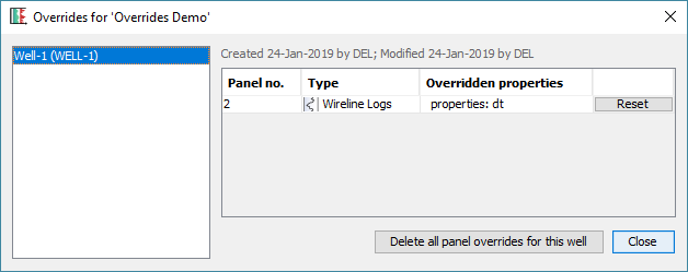
You can see which wells have overrides (and delete them if necessary) by opening the template in Charts & Templates, and selecting Chart/Template > Overrides.
In Summary
All you have to do is right-click on any templated chart block, choose Panel Properties, and then save the resulting chart. The block template will behave differently for that well, whenever you use it. You can’t change the order of panels and you can’t add or remove them – these must be done in the underlying block template.
Don’t be tempted to make the same change to a panel for each of your wells that use a template: it’s still better to change the underlying template instead.
To use this feature you will need to be running version 2.1.1. You can download this using the normal updater (select the version at the top, and make sure you get the “Latest” release), but you will need to upgrade your database as well.
New “spot cutting” sample type
The latest release of version 2.1.1 contains a new entry in the list of available sample types: the ‘spot’ or ‘bottoms-up’ cutting, SP.
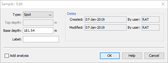
Spot cuttings are taken by pausing the downward drilling and waiting for the cuttings to arrive from the bottom of the hole. When drilling is restarted, the exact depth is known from the length of the drill string, giving a more precise depth.
The sample depth has the same precision as for a core sample since the cutting is taken from a known depth, but it is still a cutting sample.
When applying core shifts, Spot samples are shifted using the same settings for Core samples, not cuttings samples. So, if Core samples are shifted then Spot samples will be shifted. You can optionally decide whether to also shift Cuttings samples.
You can choose whether to display spot cuttings on charts. Existing samples panel templates will display SP samples in line with their setting for cuttings.
Note that in a multi-user environment, all users should update to the latest version before SP samples are added to the database, or any new samples will be seen as just cuttings.
Using SVG files in Microsoft Office
One of the consequences of moving to an integrated java based charting system in version 2.1 was that we lost the ability to generate Windows Metafiles (.wmf) from the chart program. The wmf format was a good vector based graphics format meaning that, for the graphics packages that could decode the files, the lines appeared sharp regardless of the scale it was plotted at. They were well supported by earlier versions of Windows and Microsoft Office, but more recent editions of Windows do not always render them very well. Unfortunately we have not been able to find a reliable code library that would created wmf files from our java code.
The alternatives are to create PDF files, which are vector based, or use the SVG format. The latter, which is short for Scaleable Vector Graphics, is an open graphics standard which is theoretically readable by a wide variety of software. We have found that although SVG files can be easily read by browsers like Internet Explorer, support was lacking in Microsoft Office. In Office, you needed to insert PDF files or bitmaps. These don’t always look optimal in Excel or Powerpoint.
Now, with the latest builds of Office, Microsoft have made good on their promise to be able to import SVG files. You will need a recent version – those who have an Office 365 subscription or similar will probably have received the update by now – specifically version 1705.
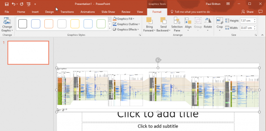
From the StrataBugs chart menus use the Export option and change the file type selector to show .SVG files. Create your file. Then in Office use the Insert Illustrations menu, select your file.
For large correlation charts which create large VGS files – particularly if you’re using logs and lithologies, the Office apps can get a bit sluggish, but otherwise it does reliably support the chart in pin sharp detail. Try it.
More information here: https://support.office.com/en-gb/article/Insert-SVG-images-and-icons-in-Office-2016-e2459f17-3996-4795-996e-b9a13486fa79
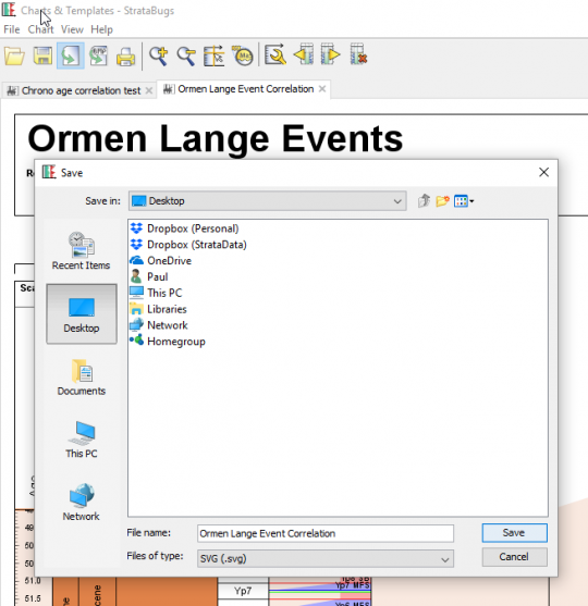
This file was 42Mb, and Powerpoint struggles, but it can read the file faithfully …
Filter by multiple categories
It has long been possible to use StrataBugs to create ‘closure’ diagrams, showing the relative abundance of different groups of species. I use the term ‘groups’ rather than ‘Groups’ intentionally, since the ‘groups’ may also be ‘categories’. A recent change has made this feature a little more flexible.
The new feature in brief
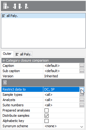
Let’s say a palynologist wants a quick overview of the relative abundance of marine vs terrestrial species. In practice this is achieved by comparing the abundance of dinocysts (category DC) with the abundance of pollen and spores (cateogry SP). Since all species belong to a category already, it’s simply a case of creating a panel which is grouped by category, and displayed as a relative stacked sawtooth plot. The only problem was that all the other palynology categories which happened to show up in the data would also be included in the plot (the left-hand panel in the image below). In the data below, the DA category represents the number of dinocysts in the first 100 specimens, so that’s what I want to compare to the SP count (N.B. your counting method might be different!).
We have now made it possible to ‘filter’ the panel by more than one category, which allows you to create the right-hand panel below comparing just DC and SP. Species not belonging to the filter categories are excluded from the data.
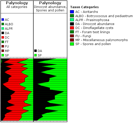
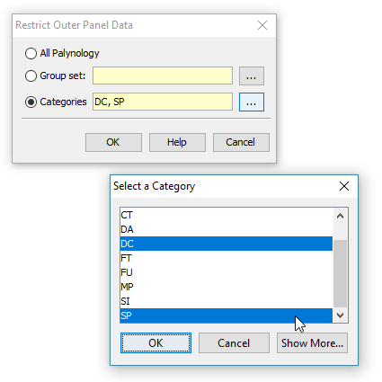
To make use of this setting, you need to select the ‘Outer’ panel properties tab, and choose ‘Restrict data to’. Here you can choose from a list of categories. To select more than one category, hold down CTRL while you select from the list.
A recap on groups and categories
All genera (and therefore species) must belong to one (and only one) category. This is a convenient way of, well, categorising taxa. Most StrataBugs users will not need to modify the standard list of categories – it would make exchanging data between databases more difficult.
Groups, on the other hand, are entirely under your control, and one species can belong to any number of groups. Groups can be attached to projects.
Both are useful for creating charts. You can find our more in the help.
More about closure diagrams
The inner panels above are created with the following options:
- ‘Group data by’ is set to ‘categories’ – this means that counts of species from the same category will be aggregated. You could also use groups here, in which case either the outer or inner panel must be filtered to a group set (which defines the selection of groups).
- ‘Plot type’ is set to ‘stacked curves’ – rather than showing the different categories in individual columns.
- ‘Calculation style’ is set to ‘relative (inner)’ which means that instead of showing the absolute count for each category, we’re showing the count as a percentage of the total for the inner panel. In this case you could also select ‘relative (outer)’ (i.e. the count is relative to the outer panel), because the inner and outer panels are showing the same data (more in this previous post).
You can find out more about the biostratigraphy panel options here.
Backup your databases
In recognition of World Backup Day (no?, me neither), a quick run through the hows and whys of backing up your StrataBugs database.
Backing up your system seems a obvious no-brainer, but take a few minutes to consider what you’re backing up, why you’re doing it, and how you might recover the database, should it be necessary.
There are two main reasons to take a backup: the most obvious being a hard drive or system failure, a fire, or theft, that results in an unrecoverable data loss. The other reason, sometimes overlooked, is the need to go back to an earlier database state in the event of accidental data loss by deleting, mistaken editing, or even a programming error (I know, I know, highly unlikley, but let’s move on..).
For the first, you need a copy – any copy – on some kind of media that isn’t the computer that StrataBugs is installed on. Most sensibly this means an external drive or memory stick that isn’t stored (and fire damaged/stolen with) the computer itself, OR, files copied ino the cloud using Dropbox or similar services. The only real pitfall of this approach is that you need to ideally make multiple copies on different media and make sure you know which ones are most up to date. In the event of a system failure you want to be able to go straight back to the most recent copy without having to try to work out which of your myriad sources of backup contained the latest database.
For users of stand-alone databases, you only really need concern yourself with the database file(s) in the /Data folder ending in .db or .mdb, since this is the only file that we can’t restore for you. All the rest of the StrataBugs files can be downloaded afresh, or supplied by us.
For users of server-based databases like SQL Server and Oracle, this backup issue is out of your hands, and one would assume that server custodians would have a backup schedule fully in place. It’s worth asking however, how often the backups are performed.
Going back to an earlier state of data is more problematic if your backup schedule always involves overwriting the previous backup copy. You might be able to recover a database, but what if you discovered a previous problem that has only just come to light, or a loss of data that pre-dates your last backup? For this reason, you should keep snapshot copies stretching back say, every day for a week, then every month for a year, then each year.
Another way to create an effective backup, particularly for server based databases, it to export the data through Organiser, or through the process that creates project databases in the Wells & Outcrops module. In this way you can selectively restore data through the usual import mechanism.
To make this process as painless as possible, a recent addition to the Connection properties dialog for H2 databases allows you to Prompt for backup:
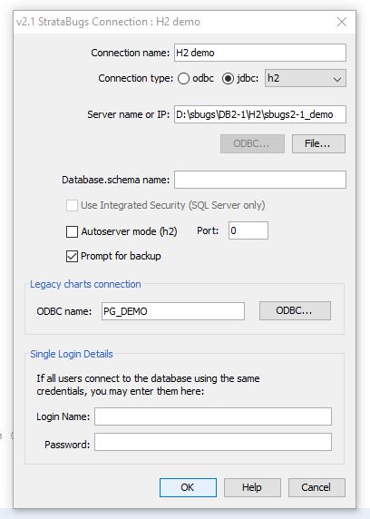
If you have this feature switched on, you will get the following dialog pop up whenever you exit from the system: 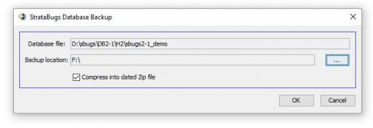
You can use this to quickly create a dated compressed backup file onto your chosen media. If you need to recover your database from the file, you need to unzip the database snapshot into the StrataBugs data folder, and provided your connection and database name are the same as the backup, you can be back up and running immediately.
Don’t let your backup be the one thing that you always meant to get around to doing … but never quite made it. If you haven’t done it recently – do it today!
Working with the Standard Chart
Amongst the many voices of approval from those that have got to grips with the templated charts in v2.1 there are always a few folks who are permanently wedded to the idea of “one well, one chart”, and don’t want to work in a templated view of the world. They also prefer a WYSIWIG panel property editor, so they can make individual panel changes as required for the well they’re working on. For them, getting to know the options available on the standard chart is where they need to start.
The Standard chart tab in the Samples & Interpretations module is always present, and contains a panel for all the data types that are present in the well. You can customise the standard chart by clicking in the chart properties icon in the toolbar: 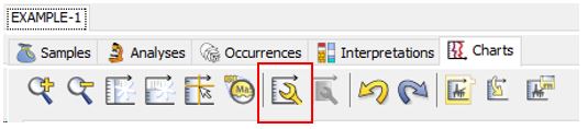 and using the panel list to add/edit and delete panels. Right clicking on any panel in the chart will bring up the option to edit the panel’s properties.
In this way you can create the chart you want. When you’re done, you can then use the rightmost button to save the chart as a template.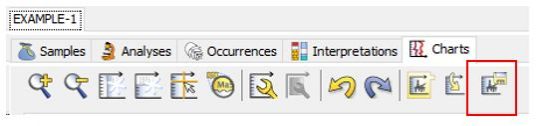
At this point you can name your template for use in the next well. Any panels that have different properties to the default will be saved in the new template.
In your second well, use the penultimate button on the toolbar to load the template you previously made into the standard chart…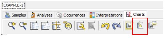
Now, make any changes you like to the panel properties. When you’re done, pres the last button again to save the template.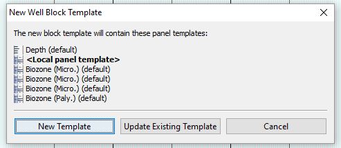 At this stage you have a choice: if you update the existing template, then this will also apply to your first well and any others that happen to be using this template. This may or may not be what you want. To keep things simple, you can select New Template, and the template name will be suffixed by the well name, and thereafter opened in a new tab bearing the template name.
When you next open your wells, the template tabs will reopen in the same state they were saved in, while the standard chart will reset to the default layout. To make changes, see above (load your template into the standard chart ….)
Lots more information on the charts tab, as always, in the help here.